An Algorithm for Local Grid Segmentation

1. Introduction

I’m building a 2D physics sandbox where hitboxes are grid-aligned. My initial approach used Box2D’s b2Chain with the Martinez-Rueda-Feito (MRF) polygon clipping algorithm to precompute chains for the entire world.

But this became impractical the moment hitboxes were added or removed.

Thus I designed LocalGridSeg, an algorithm to solve this issue using line-sweep algorithm and ghost vertex radial matching that updates ghost-vertex chains, without recomputing the entire world.

1.1 Ghost Collisions

When two polygons share a boundary, ghost collisions occur. Box2D solves this with ghost vertices: each chain segment carries references to the previous and next segment’s endpoints, allowing the physics engine to skip collisions on internal edges.

The challenge is maintaining those ghost vertices when polygons change, while doing so locally.

See Box2D’s ghost collision article for background.

1.2 Related Work

Box2D chains. Box2D represents connected edges as b2ChainSegment objects. For a chain $a \to b \to c$, segment $b$ receives ghost vertices at $a_{\text{start}}$ and $c_{\text{end}}$. Our fork exposes direct access to b2ChainSegment ghost fields.

MRF polygon clipping. The polygon-clipping library computes the union of all world polygons, producing a single non-overlapping boundary. This is correct but requires a full world recompute on every change ($O(n \log n)$ for $n$ vertices in the entire world, regardless of how local the edit is).

2. Algorithm Overview

Constraints and Assumptions

A few constraints the algo operates under; if your use case doesn’t match these, it may require adaptation.

Grid-aligned polygons. Each polygon lives entirely within a single unit grid cell $C_{i,j} = [i, i+1] \times [j, j+1]$ for integers $i, j$.

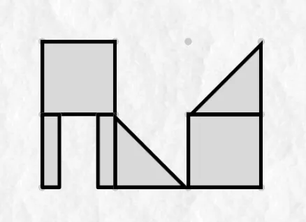
Figure 1: A grid cell containing example polygons. Each polygon is contained within its cell and may share edges with cell boundaries.

Cell occupancy. A cell is either empty or contains one or more polygons. Polygons within a cell must be non-overlapping.

Polygon properties. Polygons are simple (no self-intersections, no holes) but may be non-convex. They can have edges touching any of the four cell boundaries.

Orientation. All polygons must be oriented counter-clockwise (CCW). For any edge $\vec{e} = (e_x, e_y)$, the outward-pointing normal $\hat{n}$ is the right-hand perpendicular:

$\hat{n} = (e_y, -e_x)$

LocalGridSeg

LocalGridSeg works in two phases:

Phase 1: Boundary Segment Cancellation

When two solid cells share a boundary, their overlapping segments would produce internal collision surfaces. We run a 1D line-sweep on each affected boundary to cancel out overlapping opposite-facing segments, producing a reduced set of “resolved” segments.

Phase 2: Ghost Vertex Assignment (Radial Match)

For each vertex shared by multiple resolved segments, we reconstruct local connectivity by finding the best-matching adjacent segment.

Given an outgoing segment, we search clockwise among incoming segments sharing the same vertex; for an incoming segment, we search counter-clockwise. The best match is the segment with the smallest angular distance in the search direction.

This method allows us to assign ghost vertices correctly without needing global polygon information. Each segment’s ghost vertices are determined solely by the local radial topology at their shared vertex.

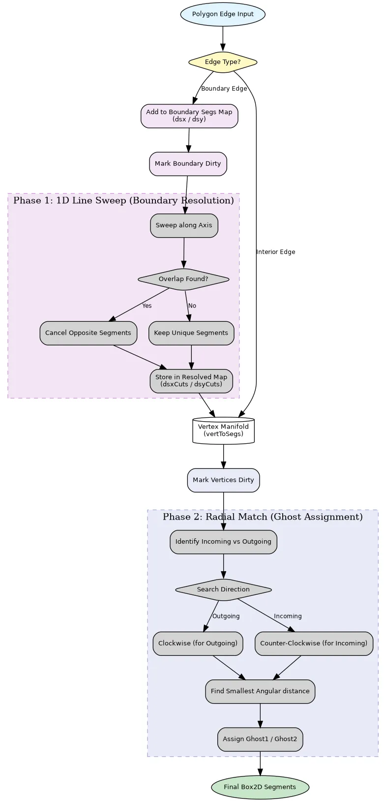
Figure 2: The lifecycle of an add/remove operation. Boundary edges flow through cancellation; interior edges go directly into the vertex manifold. The compute step processes dirty sets and produces segments with correct ghost vertices.

Data Structures

The algorithm uses five spatial maps. All are keyed by hashed positions.

(I’ll admit I definitely could have went for better variable names in the code here; so better descriptive names are used in place for explanations below)

type vec2 = [number, number];

interface Seg {
  start: vec2;
  end: vec2;
  ghost1: vec2 | null;   // previous vertex in chain
  ghost2: vec2 | null;   // next vertex in chain
  cellHash: bigint;
  ogBlock: number;       // opaque block identifier
}

vertexManifold (vertToSegs in code). Maps a vertex $v \in \mathbb{R}^2$ to every segment incident to that vertex:

$\text{vertexManifold}: v \mapsto \{ s \mid s.\text{start} = v \lor s.\text{end} = v \}$

After both phases complete, every segment in vertexManifold has correct ghost vertices and can be fed directly to Box2D.

horizontalBoundarySegs (dsx). Maps a cell position to the raw (un-resolved) segments lying on that cell’s bottom horizontal boundary. For cell $(i,j)$, the bottom boundary runs from $(i,j)$ to $(i+1,j)$. Segments here come from both the cell below (facing up) and the cell above (facing down, if present in this cell).

verticalBoundarySegs (dsy). Maps a cell position to raw segments on that cell’s left vertical boundary. For cell $(i,j)$, the left boundary runs from $(i,j)$ to $(i,j+1)$. Segments come from both the left cell (facing right) and this cell (facing left).

resolvedHorizontal (dsxCuts). After Phase 1, stores the segments that remain on a horizontal boundary after cancellation. These are the segments that get inserted into vertexManifold.

resolvedVertical (dsyCuts). Same, for vertical boundaries.

Dirty sets. Three sets track what needs recomputation:

• dirtyHorizontal - horizontal boundaries needing re-sweep
• dirtyVertical - vertical boundaries needing re-sweep
• dirtyVertices - vertices needing ghost re-assignment

---

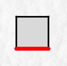
Figure 3.1: horizontalBoundarySegs for a boundary at $y=j$. Segments from the cell below face up; segments from the cell above face down.

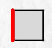
*Figure 3.2: verticalBoundarySegs for a boundary at $x=i$.

3. Methodology

3.1 Boundary Segment Cancellation (Phase 1)

Consider two adjacent cells, both completely filled. The left cell has an rightward-facing edge on the shared boundary; the right cell has a leftward-facing edge covering the exact same span. The overlapping edges are not only unnecessary, but also harmful in the way that they generate ghost collisions on what should be a seamless surface.

After cancellation, no segments remain on the boundary.

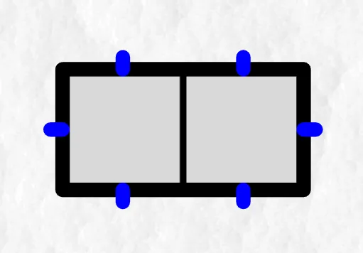
Figure 4.1: Two cells sharing a horizontal boundary with overlapping opposite-facing segments. Only the non-overlapping portions remain.

Now consider partial overlap. The left cell may have a segment from $y = 0.5$ to $y = 1.0$ (facing right), and the right cell a full-length segment (facing left). The overlapping portion from $0.5$ to $1.0$ fully cancels out, leaving only the non-overlapping portion from $0.0$ to $0.5$.

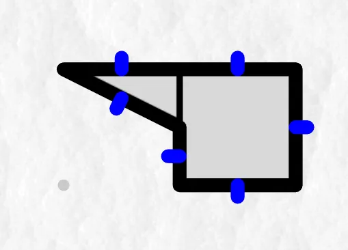
Figure 4.2: Partial overlap on a boundary. The overlapping portion cancels out, leaving only the non-overlapping segment.

For a horizontal boundary at $y = j$ belonging to cell $(i,j)$, we sweep along the $x$-axis. The algorithm is identical in concept for vertical boundaries (sweeping along $y$).

Pseudocode

function resolveHorizontalBoundary(boundaryHash):
    segs = horizontalBoundarySegs.get(boundaryHash)
    if segs is empty: return

    // Special cases: nothing to cancel
    if len(segs) == 1:
        add segment to vertexManifold, mark as resolved
        return

    if len(segs) == 2 and they exactly cancel each other:
        return  // nothing to add

    // Build sweep events
    candidates = []
    for each segment in segs:
        if segment.start.x < segment.end.x:   // faces DOWN
            candidates.push({ val: start.x, dir: DOWN, delta: +1 })
            candidates.push({ val: end.x,   dir: DOWN, delta: -1 })
        else:                                  // faces UP
            candidates.push({ val: start.x, dir: UP,   delta: -1 })
            candidates.push({ val: end.x,   dir: UP,   delta: +1 })

    sort candidates by val ascending

    // Sweep
    activeUp = 0, activeDown = 0
    results = []
    for i from 0 to len(candidates) - 2:
        curr = candidates[i], next = candidates[i+1]

        // Update active counts
        if curr.dir == UP:   activeUp   += curr.delta
        else:                activeDown += curr.delta

        if next.val == curr.val: continue  // zero-width interval

        overlapping = (activeUp > 0) and (activeDown > 0)

        if activeUp > 0 and not overlapping:
            results.push(segment from next.val to curr.val, facing UP)

        if activeDown > 0 and not overlapping:
            results.push(segment from curr.val to next.val, facing DOWN)

    // Insert results into vertexManifold and resolvedHorizontal
    for each result in results:
        add to vertexManifold (both endpoints)
    resolvedHorizontal.set(boundaryHash, results)

We convert segments into sweep events. Each segment produces a start event ($\Delta = +1$) and an end event ($\Delta = -1$). Sorting events by $x$-coordinate gives us a linear sweep.

As we sweep, we maintain activeUp and activeDown. These represent number of up-facing and down-facing segments currently covering the interval between curr and next. An interval is overlapping when both counters are positive.

For vertical boundaries at $x = i$, the same logic applies. Sweep along $y$ and track with activeLeft and activeRight.

Efficiency

The sort dominates at $O(k \log k)$ per boundary, where $k$ is the number of segments on that boundary. In practice this is fast; only dirty boundaries are swept, and $k$ is extremely small (usually 1-4 segments per boundary).

3.2 Radial Match (Ghost Vertex Assignment, Phase 2)

After Phase 1, we have a set of non-overlapping segments in vertexManifold. But segments don’t yet know their neighbors. Box2D needs each segment to know its ghost1 (previous vertex) and ghost2 (next vertex) in order to apply ghost collision handling.

Without global polygon information, how do we determine which segment connects to which at a shared vertex?

---

At any vertex $V$, segments can be classified as:

• Outgoing: $V$ is the segment’s start
• Incoming: $V$ is the segment’s end

For an outgoing segment, its ghost1 (previous vertex) should come from the incoming segment with the smallest angular distance in the clockwise direction.

For an incoming segment, its ghost2 (next vertex) should come from the outgoing segment with the smallest angular distance in the counter-clockwise direction.

Pseudocode

function assignGhostVertices():
    for each vertexHash in dirtyVertices:
        segs = vertexManifold.get(vertexHash)
        vertex = unhash(vertexHash)

        outgoing = segs.filter(s => s.start == vertex)
        incoming = segs.filter(s => s.end == vertex)

        for each seg in segs:
            isOutgoing = (seg.start == vertex)
            candidates = isOutgoing ? incoming : outgoing

            if candidates is empty: continue

            // Direction from vertex to segment's far endpoint
            farPt = isOutgoing ? seg.end : seg.start
            myDir = farPt - vertex

            // Find candidate with smallest directional angle
            best = findBestMatch(myDir, candidates, vertex, isOutgoing)
            if not best: continue

            // Assign ghost vertex from best match's far endpoint
            ghostKey = isOutgoing ? 'ghost1' : 'ghost2'
            sourcePt = isOutgoing ? best.start : best.end
            seg[ghostKey] = sourcePt

Angular Search

function findBestMatch(targetDir, candidates, vertex, clockwise):
    bestSeg = null
    minAngle = Infinity

    for each cand in candidates:
        candFarPt = (cand.start == vertex) ? cand.end : cand.start
        candDir = candFarPt - vertex

        angle = directionalAngle(targetDir, candDir, clockwise)

        if angle ≈ 0: continue     // skip self-match
        if angle < minAngle:
            minAngle = angle
            bestSeg = cand

    return bestSeg

The function directionalAngle(from, to, clockwise) computes the signed angular distance from from to to:

$\theta_{\text{ccw}} = \text{atan2}(to_y, to_x) - \text{atan2}(from_y, from_x)$

For clockwise search, the order is reversed. The result is normalized to $[0, 2\pi)$.

Worked Example

Consider a vertex at $(0, 0)$ with three segments:

Segment	Type	Direction	Normal faces
seg1: $(0,0) \to (0,1)$	outgoing	up	right
seg2: $(1,0) \to (0,0)$	incoming	left	up
seg3: $(-1,1) \to (0,0)$	incoming	down-right	down-left

Case A: Default. We search clockwise among incoming candidates (seg2, seg3):

• seg2 is at 90° clockwise from seg1’s direction
• seg3 is at ~315° clockwise from seg1’s direction

The best match is seg2 at 90°. We assign seg1.ghost1 = seg2.start = (1, 0).

Case B: seg1 is incoming, seg2 and seg3 are outgoing. We search counter-clockwise:

• seg3 is at ~45° counter-clockwise from seg1’s direction (reversed)
• seg2 is at ~270° counter-clockwise

For this case we pick seg3 at ~45°. We assign seg1.ghost2 = seg3.end = (-1, 1).

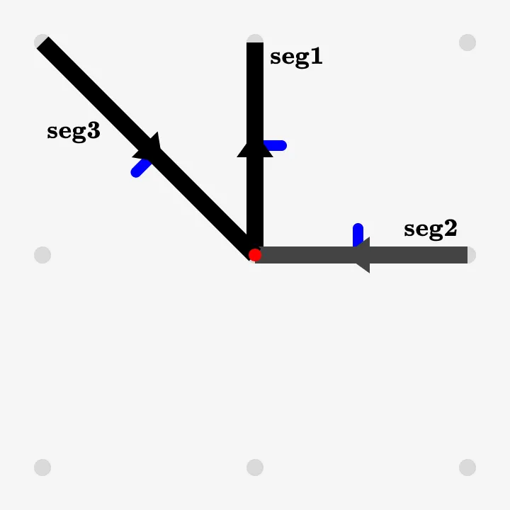
Figure 5: Three segments meeting at vertex (0,0). Blue lines represent normals of each esgment. For outgoing seg1 as described in Case A, the clockwise search picks seg2 (90° angle) for its clockwise proximity.

The example can be replicated in practice:

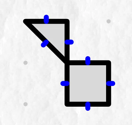
Figure 6.1: The example from Figure 5 is shown with the implementation in our physics sandbox.

And the ghost vertices of seg1 correctly assigned:

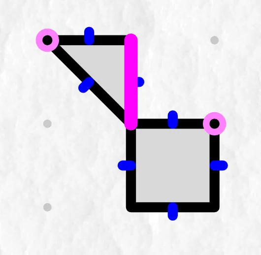
Figure 6.2: The outgoing segment (0,0) → (0,1) has its ghost1 assigned to (1,0) from the incoming segment.

4. Implementation Flow

The algorithm follows a mark-and-sweep lifecycle.

4.1 Add Operation

For each edge in the new polygon:

• If both endpoints lie on a cell boundary: the edge belongs to a boundary interface.
  • Horizontal edge at integer $y$: add to horizontalBoundarySegs, mark boundary dirty in dirtyHorizontal.
  • Vertical edge at integer $x$: add to verticalBoundarySegs, mark boundary dirty in dirtyVertical.
  • Also remove any existing resolved segments from that boundary (they’ll be recomputed).
• Otherwise (interior edge): insert directly into vertexManifold (both endpoints), mark vertices dirty in dirtyVertices.

4.2 Remove Operation

Symmetrical to add:

• Boundary edge: remove from the appropriate horizontalBoundarySegs or verticalBoundarySegs, mark boundary dirty, then cascade-remove any resolved segments that originated from that boundary:
  • horizontalBoundarySegs → resolvedHorizontal → remove those segments from vertexManifold → mark their vertices dirty.
• Interior edge: remove directly from vertexManifold, mark vertices dirty.

4.3 Compute (Boundary resolution and ghost assignment)

Called after add/remove operations. Dirty boundaries are resolved first, then dirty vertices are processed for ghost re-assignment.

function compute():
    // Phase 1: resolve dirty boundaries
    for each hash in dirtyHorizontal:
        resolveHorizontalBoundary(hash)

    for each hash in dirtyVertical:
        resolveVerticalBoundary(hash)

    // Phase 2: assign ghost vertices
    for each vertHash in dirtyVertices:
        assignGhostVertices(vertHash)

    // Clear dirty sets
    dirtyHorizontal.clear()
    dirtyVertical.clear()
    dirtyVertices.clear()

5. Benchmark Experiments & Discussion

We benchmark two scenarios with a $100 \times 100$ grid (10,000 cells).

• Scenario 1 (FullBlock): every cell contains a full-block polygon (4 vertices, 4 edges each)
• Scenario 2 (RAMP): every cell contains a randomly rotated right-triangle polygon (3 vertices, 3 edges each)

Both are measured as initialization (add-only), but removal ops are symmetric in cost since they’re equally local.

Variant	FullBlock (buildPolys)	FullBlock (initSegs)	RAMP (buildPolys)	RAMP (initSegs)
TypeScript	11.73 ms	29.02 ms	9.57 ms	43.44 ms
Baseline C++	1.26 ms	5.28 ms	0.85 ms	23.28 ms
Optimized C++	0.91 ms	3.87 ms	0.68 ms	18.42 ms

buildPolys is the time to generate polygon vertex data. initSegs is the time to run the full LocalGridSeg algorithm (both phases).

The RAMP case is slower than FullBlock because non-boundary edges create more entries in vertexManifold, increasing ghost-vertex assignment work.

5.1 Performance Characteristics

The C++ ports demonstrate significant headroom in comparison to the original, unoptimized TypeScript implementation. Baseline C++ is a direct 1:1 port with equivalent data structures (std::unordered_map, std::vector). Optimized C++ replaces general-purpose hash maps with fixed-size arrays and bit-packed vertex representations to eliminate allocations and hash computations.

5.2 Implementation Notes

Floating-point hashing. Vertices are hashed by reinterpreting their Float32 bit patterns as BigInt in JS, and uint64_t in C++. This ensures two vertices either have identical float bits (or they don’t). We use an epsilon only for equality comparisons (e.g., vec2Equals with $\epsilon = 10^{-3}$) to handle potential fp drift.

The shouldPreserve flag. The implementation includes an optional callback shouldPreserve(block1, block2) that, when returning true, prevents cancellation of overlapping segments even when both directions are active. This is useful when segments belong to different “materials” that should maintain separate collision surfaces. For the standard case, assume it always returns false.

6. Conclusion and Future Work

LocalGridSeg is a practical algorithm for maintaining ghost-vertex chains on grid-aligned polygons under dynamic updates. By exploiting the grid structure and reducing the problem to local boundary sweeps and radial vertex matching, it achieves update costs proportional to the size of the change rather than the world.

We have applied and validated the algorithm in our physics sandbox, marblebuilds, and handles thousands of dynamic polygons at interactive framerates.

6.1 Future Directions

• Non-grid-aligned polygons. Relaxing the grid alignment constraint while maintaining the non-overlapping guarantee.
• Bulk full-block optimization. When large contiguous regions of full blocks are added/removed, the boundaries cancel entirely.
• Generalization. The radial match technique may apply to other problems where local manifold reconstruction is needed from directional edge sets.

Dependencies

• Box2D v3+ physics engine with ghost vertex support
• Box2D documentation